Line Control

Sensor Configuration

Naturally, the main sensors used for staying within the line boundaries are the light sensors. We have 36 light sensors arranged in a ring, as well as 2 extra light sensors at the left and right. While the 2 extra sensors can be used for early detection of the lines, we did not actually end up utilising it in our staying within bounds strategy.

Light sensor ring

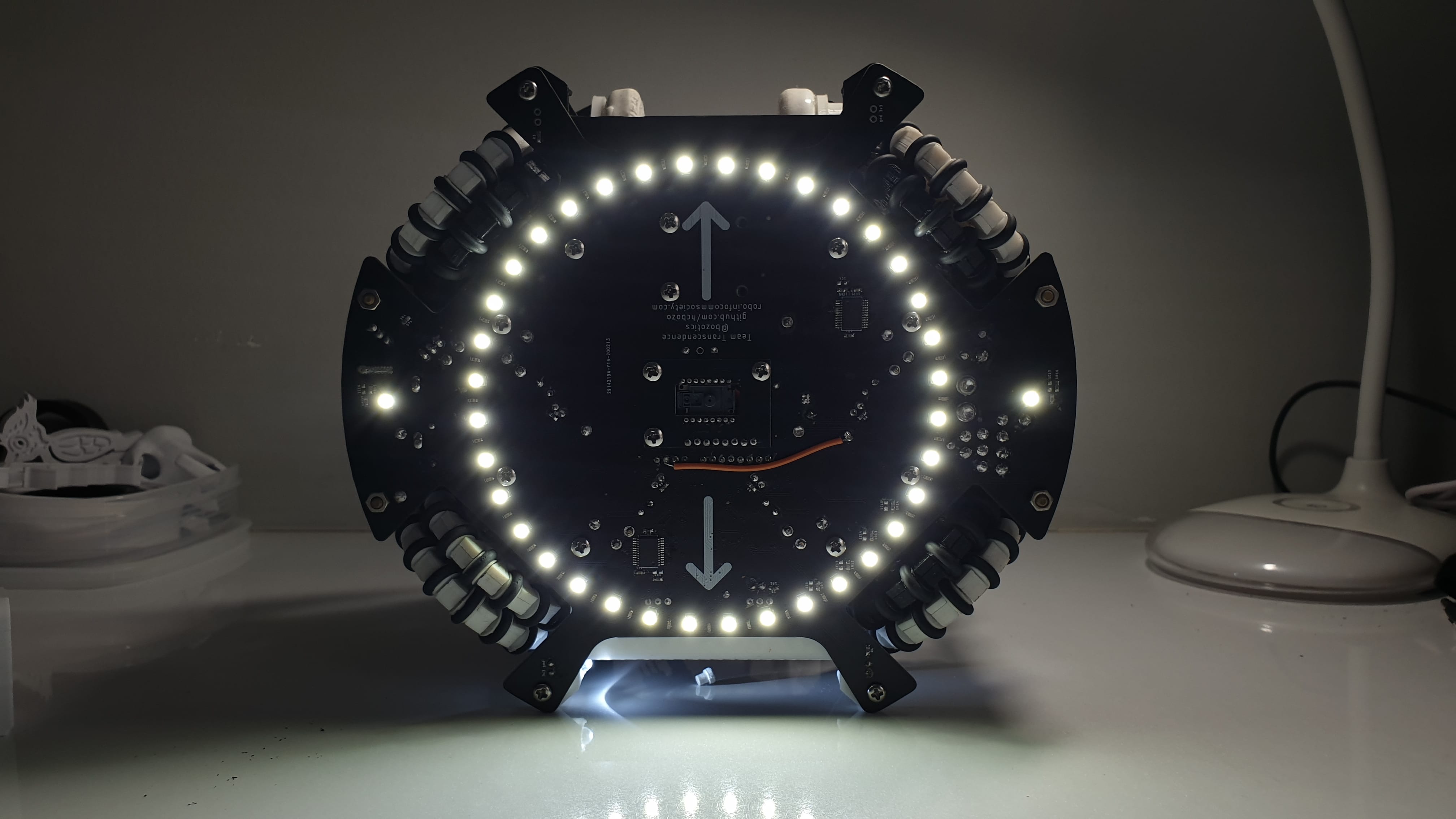
We opted for 36 for ease of programming, so that each sensor simply represents 10 degrees (measuring from the centre of the robot). Theoretically, any number of sensors and any shape of configuration will work with our strategy as long as there is a connectable ring of light sensors and the angle to each of them is known.

In addition, since the camera is able to tell us the vector to the centre of the field (see Localisation), we can also use it to tell how close we are to the edge of the field, as well as the position of the line relative to the field, which could be useful to tell when it is safe to stop avoiding the line and start tracking the ball again.

Line Avoidance

Being able to stay in the field is top priority, on par with being able to follow the ball, because once any robot leaves the field, the team will be at a severe 2-to-1 disadvantage for a full minute. Hence, we can rely on staying in-bounds purely through our light sensors, which means it is essentially impossible for outside interference to ever affect our robot’s ability to stay in-bounds.

Do note that “Line Avoidance” refers to the motion of moving away (typically in a perpendicular direction) from the line, back towards the field, i.e. rejecting the line.

Light Sensors

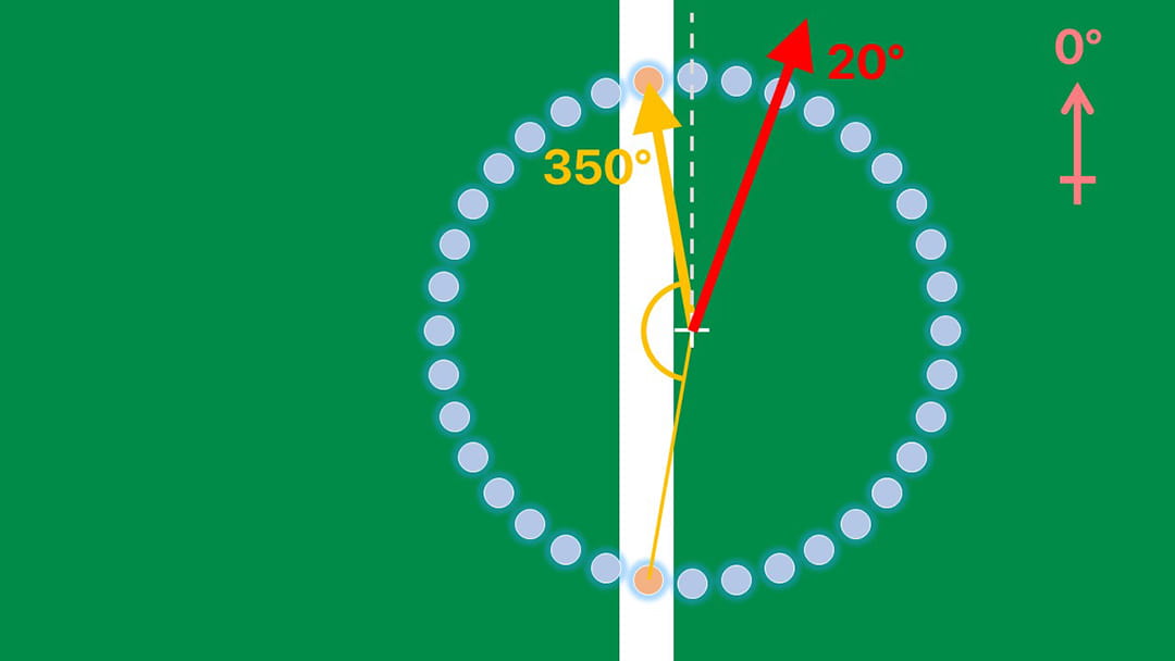
Since the light sensors are in a ring, when the robot first touches the line, there will be clusters of sensors that show up as detecting the presence of the white line. We take the 2 sensors that give the biggest non-reflex angle about the robot’s centre. Finding the angle bisector of these 2 sensors will give the angle that is perpendicular and towards the line, from the robot’s centre. This works regardless of what type of line the robot is on, as shown in the diagrams below.

Light ring on different types of lines

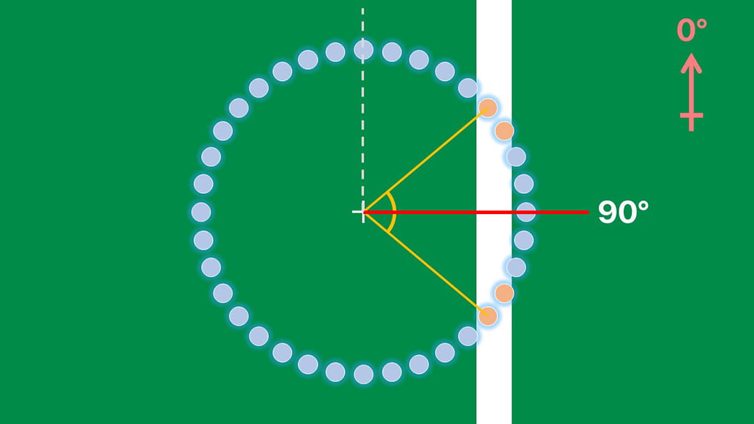
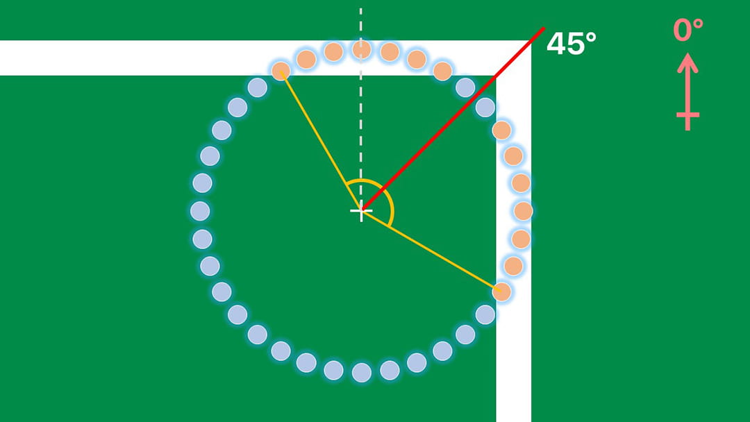
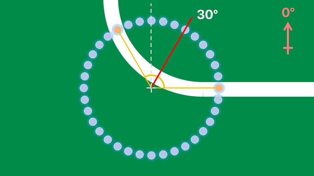
We can also determine the relative length of the chord that crosses these 2 sensors, normalising it between 0 and 1 where 1 is the diamemter length. This chord length is a proxy measurement of how much the robot has crossed over the line. Hence the speed of the robot’s rebound is proportional to this chord length.

Chord length increases as robot moves over line

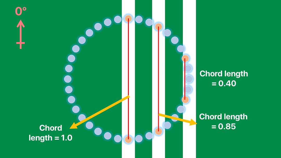
However, when the robot crosses the halfway mark, the chord length will begin to decrease, so how do we continue using it to measure how much the robot has crossed the line? Well, since the angle bisector cuts across the non-reflex angle, when the halfway mark is crossed, the angle bisector will essentially “flip” to the other side. Hence, when there is a huge jump from the previous angle of the angle bisector to its present angle, we know the robot is more than halfway past the line and we modify the chord length variable to continue increasing above 1, all the way up to 2.

Hence, “mathematically speaking”, when the smallest angle difference between A_initial and A_present is larger than 90°:

$R = \left\{ \begin{matrix} A_{present} + 180\degree & f(A_{initial},A_{present}) \leq 90\degree \\ A_{present} & f(A_{initial},A_{present}) > 90\degree \end{matrix} \right.$ $L = \left\{ \begin{matrix} \mathit{l} & f(A_{initial},A_{present}) \leq 90\degree \\ 2-\mathit{l} & f(A_{initial},A_{present}) > 90\degree \end{matrix} \right.$ $S_{present} = L \cdot S_{default}$

where R is the robot’s bearing to move away from the line, A is the angle of the angle bisector, l is the chord length between the sensors, L is the modified chord length variable representing how far off the line the robot has gone, S is the robot’s speed, and f(x,y) is a function that returns the smallest angle difference between the 2 parameters in degrees.

Incorporating Camera

An alternative to a pure light sensor line avoidance is to use information about the location of the centre point of the field. The most simplified method would be to move in the direction of the centre of the field when a line is detected. However, this may be too simplistic as there is over-reliance on the camera data which has a higher chance of interference.

Robot moves in direction of field centre when it hits a line

A better way could be to find both angle bisectors (of the reflex and non-reflex angle) and move in the one that more closely matches angle to the centre of the field. This simplifies the program as it eliminates the need to check for the “flipping” of angle bisectors.

However, we feel that the simplification which using the camera data brings about does not justify the decreased robustness of the line avoidance program, which is why we still rely on pure light sensor for line avoidance.

Uses

This is mainly used when the robot hits a line at a high speed. Direct line rejection is necessary to ensure the robot cancels out all the momentum built up from travelling to the line at its high velocity. However, constantly doing line avoidance would result in unnecessary oscillations about the line, which is where the 2nd approach to line control comes in.

Line Tracking

This is the process where the robot moves to an object/in a certain direction while following a line.

Theory

As with “normal” (think: 2-wheeled WRO robot) line tracking, there must first be a desired direction to travel in. This is dependent on what object the robot is trying to chase (e.g. ball, goal, point on field).

Next, the robot finds the light sensor that is closest to the desired angle. The angle of this light sensor will thus be the direction of the robot.

Various line track angles based on desired angle of 20°

As for speed of the robot, it varies inversely with the chord length (i.e. it moves faster the further it is from the halfway mark of the line) as well as inversely with the perpendicular angle deviation of the ball (i.e. it slows down). Hence, the equation for the robot’s speed is:

$S_{present} = \min(S_{max}, a \cdot \sqrt{D} + b \cdot \mathit{l})$

where S_max is the preset maximum speed of the robot, D is the angle of deviation from how far the ball is to being perpendicular to the robot, l is the chord length, and a, b are constants to be tuned.

Incorporating Camera

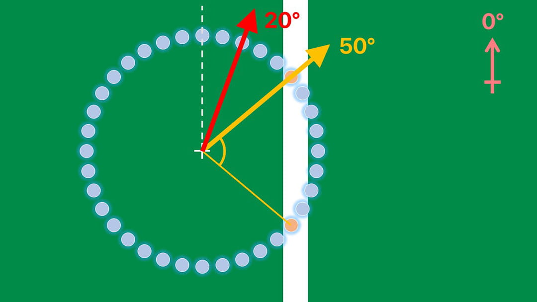
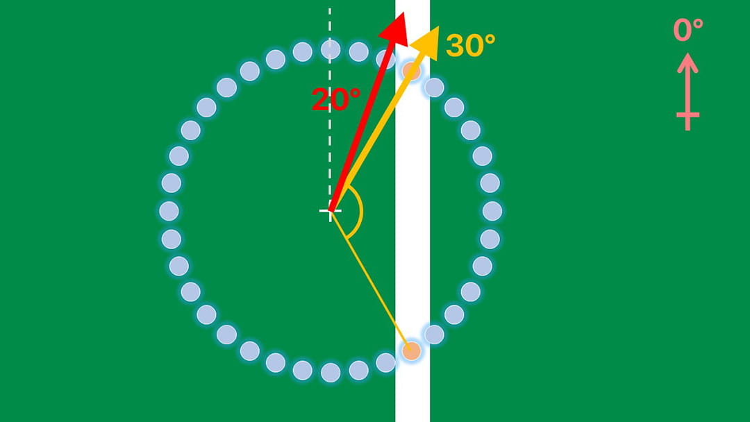
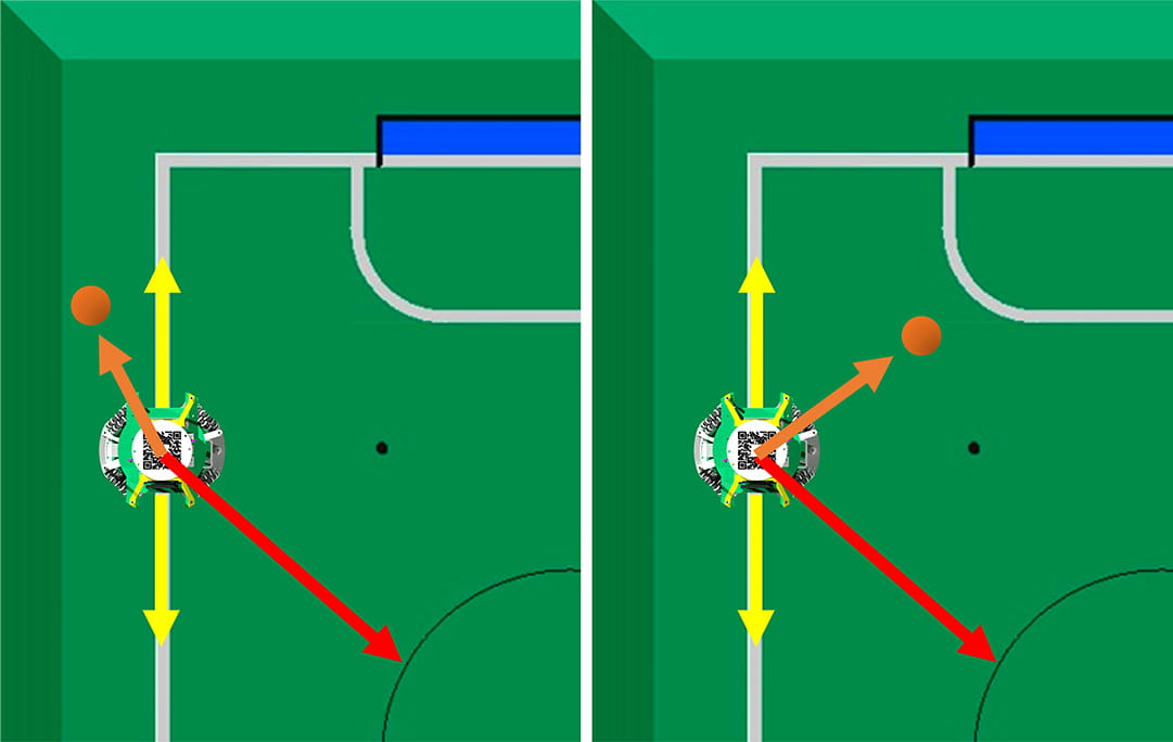
When using line tracking to stay within the field, the location data is used to tell when the ball has been returned to the field. As shown in the diagram below, the yellow arrows represent the angles of the 2 sensors that are detecting the line, the red arrow represents the direction to the centre of the field and the orange arrow is the ball angle. With the yellow arrows acting as the half line, as long as the red and orange arrows lie on the same half it is safe to continue ball chasing.

Robot moves in direction of field centre when it hits a line

A non-localisation based method can work by recording the last seen ball angle and where the robot came from, and then checking whether the ball presently lies on the same side as the robot. This would reduce the reliance on the localisation data, a possible point of inaccuracy. However, we have not gone for this solution yet solely because we’ve been too lazy to program that lmao. ~kfc

TO BE UPDATED!

Uses

Line tracking is used in many places, to stay within bounds, for going to points on the field that lie on the line, and for the goalie program to track the penalty area line.

A very obvious AFI would be to implement PID line tracking, not just the proportional line tracking method currently used, but again sorry i lazy. ~kfc